
Python challenge 2 - How do computers recognise songs?
How can a computer recognise a song? Everyone has seen it: a snippet of a song is recorded on a phone, then after a few seconds it recognises the song that is playing. This week, we consider how humans (and machines!) can recognise songs using a Spectrogram.
How do computers recognise songs?
Sound waves are recorded by a microphone as a series of numbers. These signals can therefore be plotted. However, it is actually quite challenging for a human (and even a computer) to analyse all of the information in one go just by using that information.
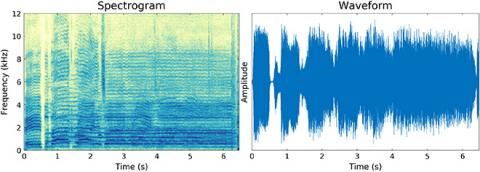
A common approach is to look at the frequency content of a signal (the `spectrum'). This is done by chopping the signal into sections, and then calculating the Fourier Transform of the chopped up signal. Putting all of the chopped up frequency content together creates a Spectrogram of a song. This week's program will produce a spectrogram of a song, as below.
Target:
Write one page of Python that will:
- Load a song, and then have Python play the song back to you.
- Plot the waveform of the song.
- Plot the logarithm of the spectrogram of your song, against time and frequency.
Extensions:
- When you calculate and then plot the frequency data, experiment by increasing the time resolution. What do you notice about the `sharpness' of the frequency if you reduce the time step?
- What you observe is related mathematically to a well-known physics phenomenon. Can you identify which phenomenon it is related to?
- A paper detailing a popular song-search algorithm is freely available online. Can you find this paper? How does it use a spectrogram to find songs?
Try to get as far as you can on your own before viewing the hints or the solution
-
Hints for Python Challenge 2
The easiest way to manipulate audio data is as a '.wav' file.
Packages
In this solution to this problem, pygame can be used to play sound. The scipy packages has modules for loading '.wav' sound files within scipy.io, and scipy.signal has a method to create a spectrogram.
Within matplotlib the contourf function is used to plot the spectrogram above. Try experimenting with different colourmaps (using colormap within matplotlib).
Hints
- It can be quite tricky to find the path to a file sometimes. On a first run, the easiest way to open a file may be to specify the path directly, but it is best practise to append paths to sys.path.
- Often a wav file will be in `stereo', so the sound is in two channels (left and right). A single signal can be found for analysis either by finding the average of these two signals (for example using numpy.mean) or each channel could be chosen individually.
- The data that is read in from scipy.io is for a whole song. What time does each entry of the array count for? It is helpful to only select a few seconds of the song to analyse, because each file is large.
- The output of the spectrogram is in the form of 'complex numbers'. To convert to find the 'magnitude' of the response, which we are plotting, use the 'abs' function within numpy.
- When plotting the spectrogram, sometimes the range is too large to get a nice picture. Adding 1 to all points in the logarithm (for example, Z = np.log10(np.abs(spect) + 1)) sometimes makes figures more clear by ignoring very small responses.
Notes
Sound is perceived on a logarithmic scale with frequency. That is, doubling the frequency increases the pitch of a note by one octave. Plotting the spectrogram with a logarithmic frequency scale (using, for example, plt.gca().set_yscale('log') may therefore make the spectrogram more intelligible, and also highlights low notes better than if a linear scale from 0 to 22 kHz is used (human hearing is approximately 0 to 20 kHz).
-
Solution for Python Challenge 2
# ===== Challenge 2: How do computers recognise songs?

import os, time, pygame, sys
import matplotlib.pyplot as plt
import numpy as np
from scipy.io import wavfile
from scipy.signal import spectrogram
from matplotlib import cm

# Get the current directory
working_dir = os.path.dirname(sys.argv[0])

# 1: Load a song and play it back.
fn = os.path.join(working_dir, 'paperback_writer.wav') # <-- Path to a wav file here
pygame.mixer.init()
# There are a number of different packages to play audio;
# pygame is one example.
song = pygame.mixer.Sound(fn)

song.play()
time.sleep(8)
song.stop()

# 2. Load the song as a wavfile.
samplerate, data = wavfile.read(fn)

# Start and end time in seconds
t_start = 0.5
t_end = 7

n_start = int(t_start * samplerate)
n_end = t_end * samplerate
t = np.linspace(t_start, t_end, n_end - n_start)
# Get the sample
sample = np.mean(data[n_start:n_end], axis=1)

# Plot the waveform
fig,ax = plt.subplots()
ax.plot(t - t[0], sample/np.max(sample), linewidth=0.3)
ax.set_xlabel('Time (s)')
ax.set_ylabel('Amplitude')
ax.set_xlim((0, t[-1]))
ax.set_title('Waveform')
ax.set_yticks([])
plt.tight_layout()
plt.show()

# 3. Calculate and plot the spectrogram.
nBits = 10
fs, ts, spect = spectrogram(sample, samplerate, nperseg=2**nBits)

fig,ax = plt.subplots()
ax.contourf(ts, fs/1e3, np.log10(abs(spect) + 0.1), 20, cmap=cm.YlGnBu)
ax.set_ylim((0.0, 12)) # kHz
ax.set_xlim((0.0, ts[-1])) # kHz
ax.set_xlabel('Time (s)')
ax.set_ylabel('Frequency (kHz)')
ax.set_title('Spectrogram')
plt.tight_layout()
plt.show()
Ready for the next challenge?
Click here to explore 'How fast a computer can read all of Wikipedia'